Stationarity helps us to understand what strategies suit a market statistically. Stationarity shows how often prices revert to mean value.

If stationarity is high, we can trade mean-revert strategies. If it is low - trending systems work better.

I will show how to calculate stationarity for all markets in the dYdX exchange.

To make calculations, we need a casual OHLCV. Large timeframes are better for seeing the big picture, as the situation in tiny timeframes changes too fast.

TIMEFRAMES = ['1DAY', '4HOURS', '1HOUR', '15MINS']

After we receive OHLCV, we can calculate stationarity in one line of code with statsmodels!

result = adfuller(df.close)

It is easy to understand the result. If the p-value is less than 0.05, our prices are stationary.

print('p-value: %.2f' % result[1])

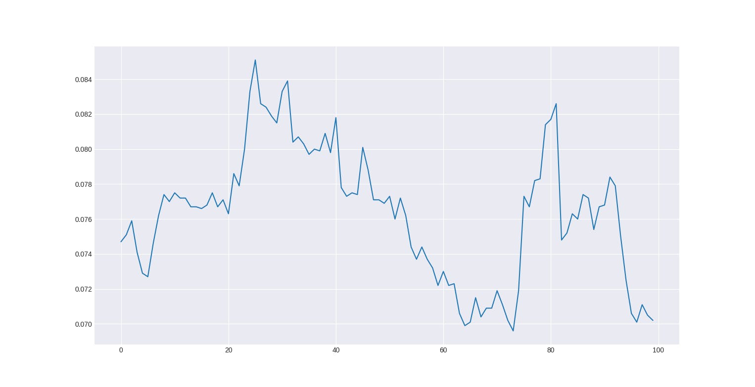
Some examples. Stationary prices:

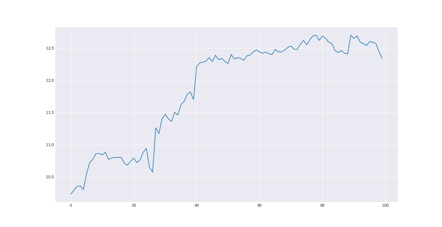
Non-stationary prices:

We can also take p-values from several timeframes and add and then select the largest and the smallest values to find out what markets tend to be more trending.

The most trending markets: $MATIC, $AVAX, $CRV.

The least trending markets: $UMA, $CELO, $ETC

The difference between the two groups is between 2 and 3. It can't guarantee a positive result, but it can help to select more optimal markets for a particular strategy or to filter a signal with this data.

GitHub repo - https://github.com/Jungle-Sven/stationarity

Twitter - https://twitter.com/jungle_sven

#algotrading #statarb #timeseries #stationarity